
In this blog, we investigate the performance of direct solvers in COMSOL Multiphysics across a range of CPU and GPU systems using eight representative benchmark models. The study compares MUMPS, Pardiso, and cuDSS across different hardware classes, operating systems, and memory configurations in order to identify the factors that most strongly influence runtime.
The results show that GPU acceleration can provide substantial speedup, but the benefit is highly model dependent and requires the problem to fit within available VRAM. Even when running models on the GPU with cuDSS, the CPU capability, RAM, and operating system also have a significant impact on performance, and a balanced system design is often more important than maximizing any single hardware metric.
Overall, the study shows that GPU can give significant speedup but that reliable performance in COMSOL Multiphysics® is model and physics dependent and that benchmarking on real application workflows is necessary rather than relying only on synthetic tests.
Introduction
Graphics processing unit (GPU) acceleration is increasingly important for large-scale finite-element simulations, but the practical benefit in COMSOL Multiphysics depends strongly on model type, solver choice, and hardware configuration. While modern GPUs offer substantial computational throughput, real-world COMSOL performance is determined by the interaction between solver implementation, central processing unit (CPU) capability, memory capacity, operating system, and the numerical structure of the model being solved.
This blog investigates how direct-solver performance changes across a range of representative COMSOL workloads and hardware platforms. The study focuses on MUMPS (multifrontal massively parallel sparse direct solver), Pardiso, and cuDSS (CUDA Direct Sparse Solver), with particular emphasis on when GPU acceleration provides meaningful speedup and when conventional CPU execution remains competitive. Rather than relying only on synthetic benchmarks, the analysis is based on eight application-oriented models spanning transport, thermal, and structural mechanics problems.
The goal is to identify the hardware and software choices that matter most in practice. In particular, we compare CPU and GPU behavior across different system classes, examines the effect of operating system choice, and highlights the role of random-access memory (RAM) and video random-access memory (VRAM) limits in determining whether a given configuration delivers useful acceleration. Together, these results provide a practical basis for selecting systems for COMSOL workflows that rely on large direct-solver workloads.
Methods and Evaluation Criteria
We evaluate solver performance across a range of hardware platforms. The three primary solvers tested in this study are MUMPS, Pardiso, and cuDSS. We focus on direct solvers because, as of COMSOL 6.4, GPU acceleration has been implemented within this part of the solver architecture. The main comparative analysis therefore focuses on direct-solver workflows. The SolarPanel model is retained as a reference case for consistency checks across systems, but because it uses an iterative multigrid solver rather than MUMPS, Pardiso, or cuDSS, it is not interpreted as part of the direct-solver comparison in the same way as the other models.
Testing different solvers on the same models and systems allows us to evaluate both solver-specific speedup on an individual machine and performance differences between systems.
The investigation was carried out using compiled COMSOL applications in order to distribute the benchmark efficiently across many systems. All benchmarks were run using COMSOL Multiphysics 6.4, build 378, with the same application compiled for Windows, Linux, and Linux Arm. For each model, three phases were recorded: model building, solving, and postprocessing. The eight models were then run in series while the time required for each phase was recorded.
Each benchmark configuration was typically run once for the reported results. Consistency checks were performed intermittently by repeating selected runs, and these repeat runs showed run-to-run variations of approximately 2%. Since this variation was small relative to the larger differences between systems and solver configurations, we report single-run timings rather than averages over repeated runs.
The times are then compared across solvers and systems to obtain the speedup metrics used throughout this post.
When a configuration forced the solver into out-of-core execution because the model did not fit in available memory, the corresponding data point was marked in gray and excluded from average-performance calculations.
Model Setup
Eight models were used. They were selected to provide a diverse set of physics interfaces, model types, and study types. Most were taken from the COMSOL Application Gallery and modified to fit the specific benchmarking requirements. In general, the direct solvers MUMPS, Pardiso, and cuDSS were selected as described in the corresponding table entries below.
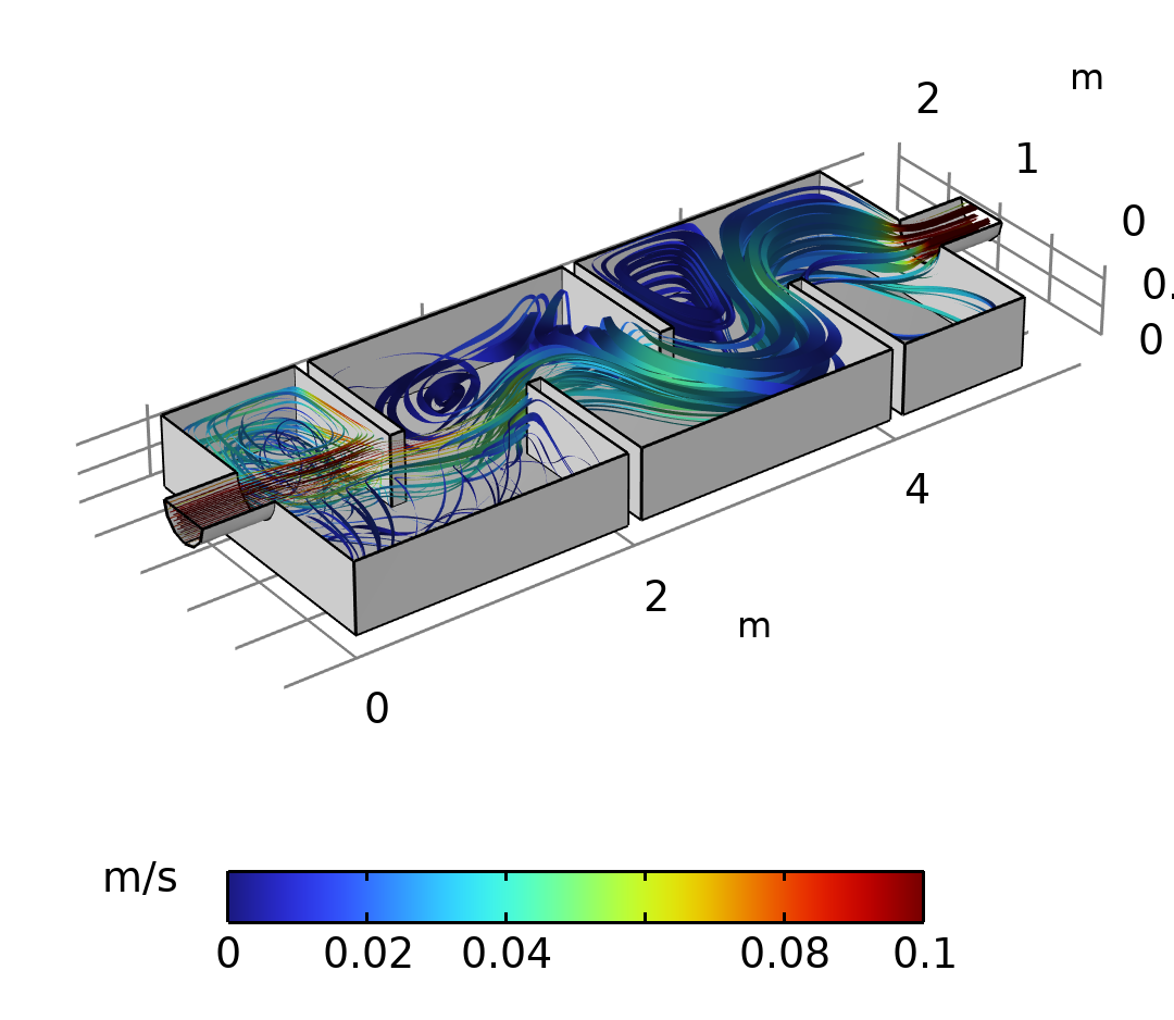
1. Water purification reactor
This benchmark represents a reactor-transport application and is included to capture solver behavior on a chemically motivated multiphysics model. It provides a useful comparison point because it differs substantially from the structural and thermal examples elsewhere in the benchmark suite. The Application Gallery source used for this case is available from COMSOL at water-treatment-basin-14049.
The model uses a k-ϵ formulation to calculate turbulent flow in the basin. It is a stationary study that uses a segregated method with direct solvers.
2. Cohesive zone debonding
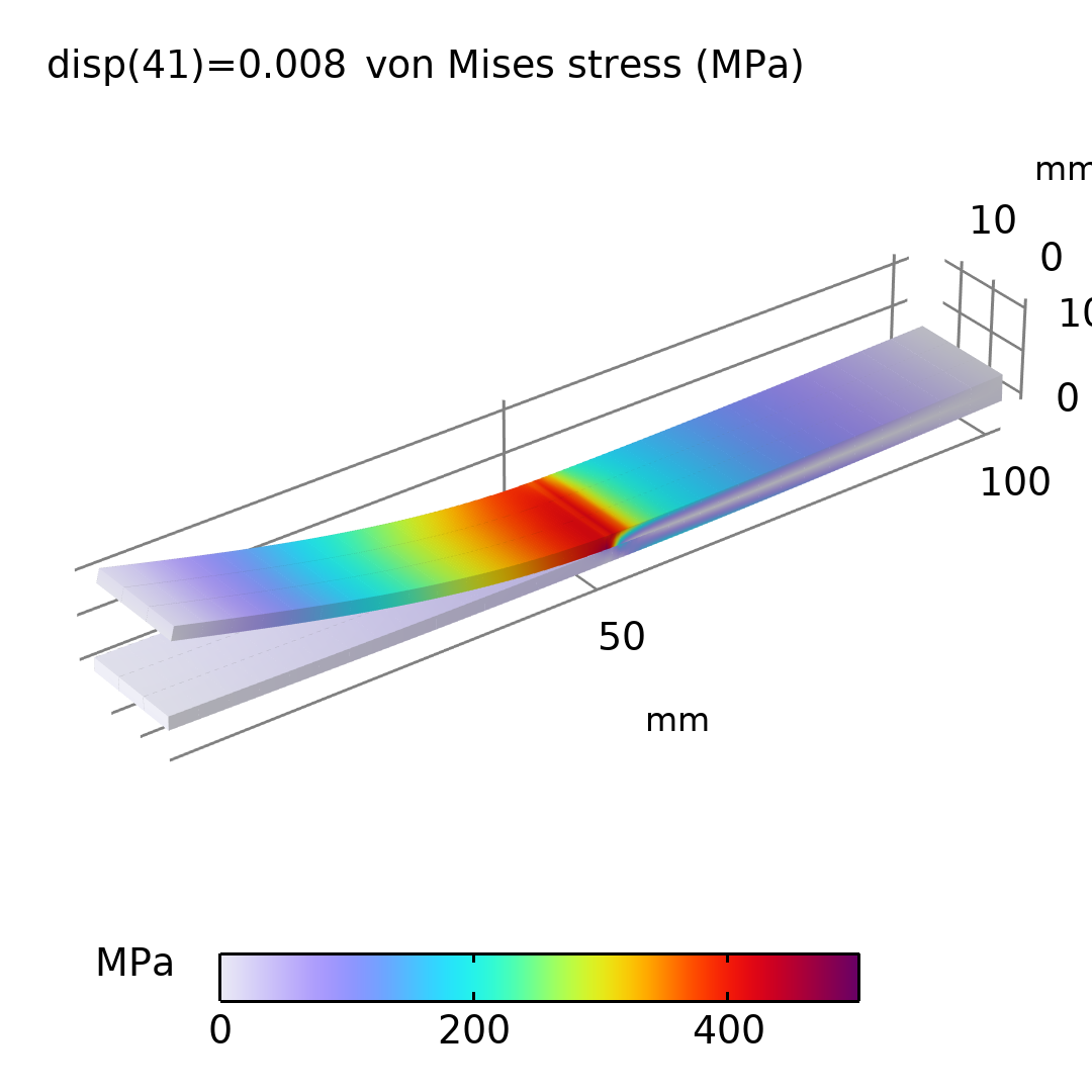
This model captures interfacial fracture behavior in a laminated composite and provides a useful structural-mechanics benchmark with strong contact-like characteristics. It broadens the benchmark suite by stressing solver robustness on a mechanically complex problem rather than on transport- or heat-dominated physics alone.
The Application Gallery source used for this case is available from COMSOL at mixed-mode-debonding-of-a-laminated-composite-19961, and it is included here as one of the representative models for comparing runtime trends across architectures and solver choices. The physics consists of linear elasticity with adhesion and loading applied at the cracking edge. It is a stationary study with an auxiliary sweep in displacement. The solution uses a fully coupled method and a direct solver.
3. Thermal bridge 3D iron bar
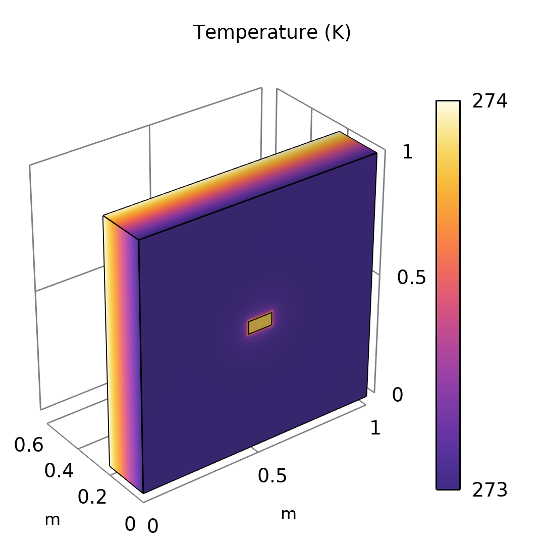
This benchmark introduces a building-physics heat-transfer case with clear geometric conduction paths and material contrasts. It helps test how solver performance changes on a thermal model with a very different sparsity pattern and coupling structure from the reactor and fracture examples. This model is also relatively small and solves quickly, thereby providing an indication of overall system responsiveness and performance on small models.
The COMSOL Application Gallery source for this case is thermal-bridges-in-building-construction-3d-iron-bar-through-insulation-layer-12575, and it is used here to represent steady thermal analysis within the benchmark suite.
The physics is heat transfer in solids with a stationary study, a fully coupled method, and a direct solver.
4. Laplace’s equation model
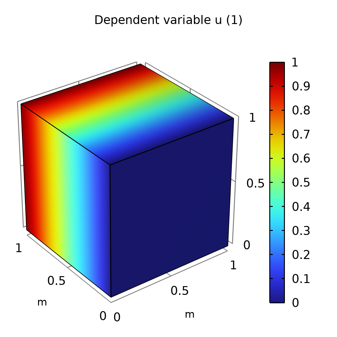
Laplace’s equation model is a deliberately simplified benchmark designed to isolate raw solver throughput from application-specific modeling complexity. The model uses a cube geometry, a single weak-form equation corresponding to Laplace’s equation ∇²f = 0, Dirichlet boundary conditions on two opposite faces, and zero-flux conditions elsewhere.
To make the case computationally meaningful, the mesh is refined until the model consumes roughly 30 GB of memory and requires a measurable solve time. This makes it useful as a controlled reference case for comparing direct-solver behavior, including cuDSS-enabled execution, under heavy linear-system load. This model is the only one that reaches full GPU utilization while solving. It uses a stationary study, a fully coupled method, and a direct solver.
5. Electronic enclosure cooling
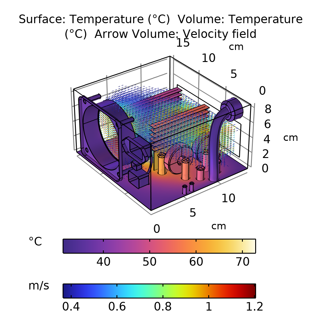
This model adds a forced-convection thermal-management problem to the benchmark set and is intended to capture solver behavior on a coupled flow-and-heat-transfer application. It complements the other cases by representing a more engineering-oriented enclosure-cooling scenario with fan-driven transport effects.
The COMSOL Application Gallery source for this benchmark is forced-convection-cooling-of-an-enclosure-with-fan-and-grille-6222, and it is included to broaden the evaluation across practical multiphysics workloads.
The physics interfaces are “Heat Transfer in Solids and Fluids” and “Turbulent Flow, Algebraic yPlus.” The study is a two-step process: the first step is a “Wall Distance Initialization,” and the second step is a stationary solver. Both steps use fully coupled methods and direct solvers.
6. Rim Sub model
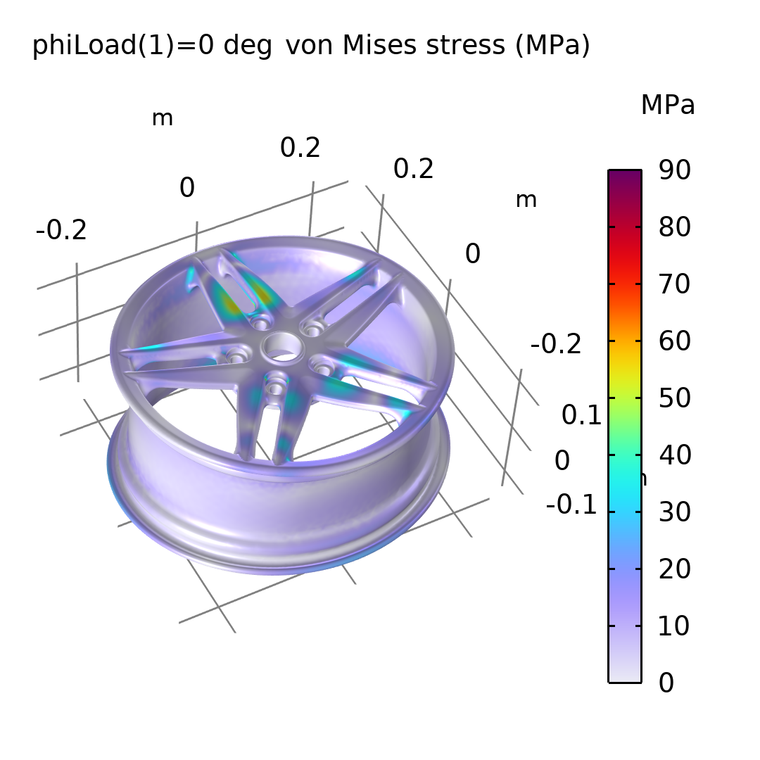
RimSubmodel represents a structural submodeling workflow and is useful for assessing solver behavior on localized high-fidelity mechanics problems. It introduces a different balance between global context and local resolution than the full-domain examples, which can affect both factorization cost and memory behavior.
The source application used for this benchmark is submodel-in-a-wheel-rim-8517, and it helps capture solver performance on a realistic structural-engineering case. The model consists of two components, both using linear elasticity, one solving for the full model and one as a submodel of the rim. Both use auxiliary sweeps and stationary solutions with fully coupled methods and direct solvers.
7. Sheet Metal Forming
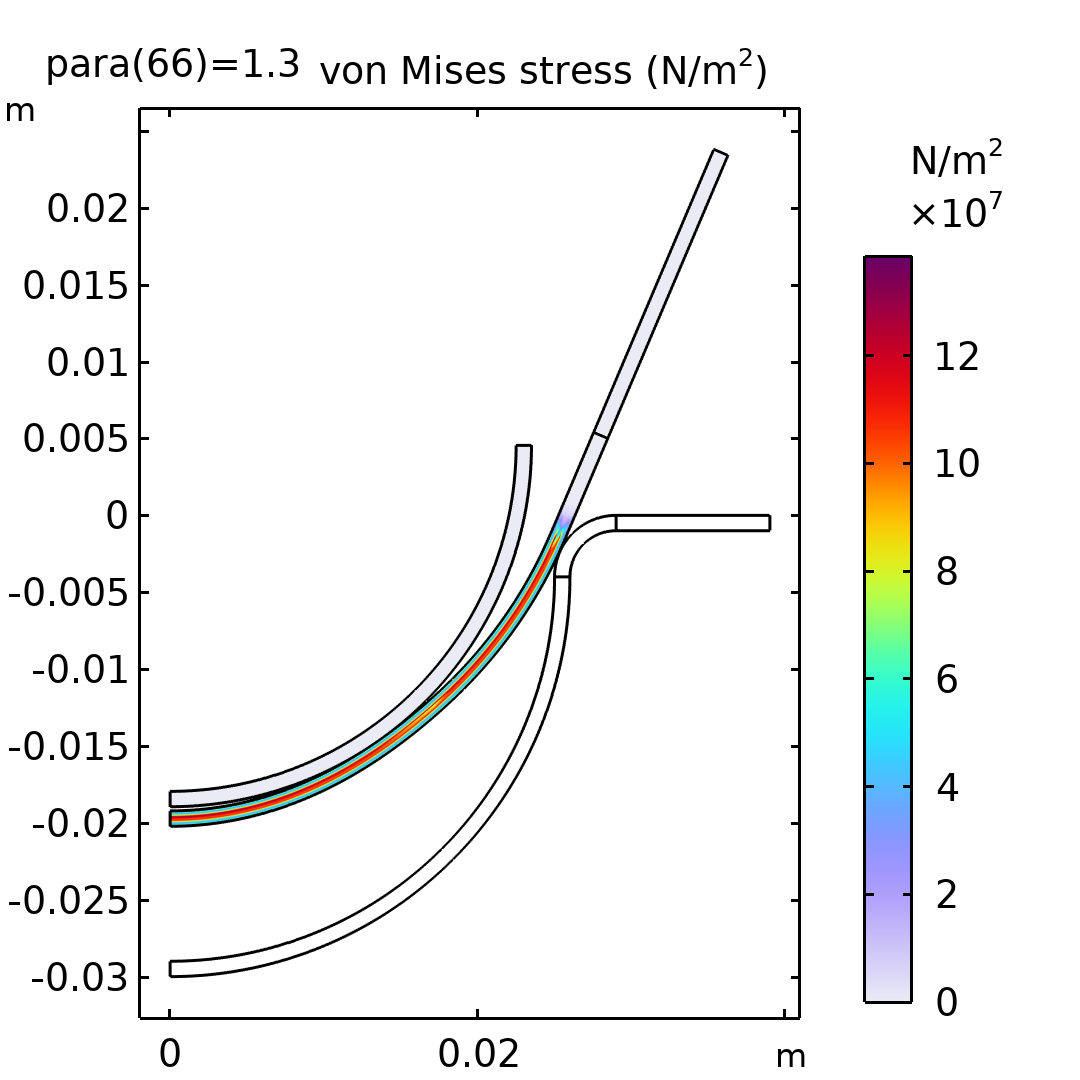
This benchmark extends the suite into deformation-dominated manufacturing simulation. Sheet-metal-forming problems are valuable in the comparison because they can involve dynamic contact effects and large structural responses, both of which place different demands on the solver stack than the thermal and transport models.
The Application Gallery reference for this case is sheet-metal-forming-11208, and it is included to represent structural processing workflows in the study.
The model has two components: a 2D solid-mechanics component and a 3D shell-physics component. There are three studies, all with stationary study steps, in which the punch displacement is calculated through auxiliary sweeps. Two of the studies use segregated methods, and one uses a fully coupled method; all use direct solvers.
8.Solar Panel
The solar-panel model provides a coupled application with flow interaction and device-scale thermal behavior, helping extend the benchmark beyond purely mechanical or conduction-focused cases. It is useful as a contrasting workload because it is configured with an iterative multigrid solver. It is not set up for switching between direct solvers and therefore serves primarily as a comparison and consistency check across runs rather than as part of the main MUMPS, Pardiso, and cuDSS benchmark set.
The COMSOL Application Gallery source is solar-panel-in-periodic-flow-12205. In this study, the model primarily serves as a reference case for workflows that remain outside the MUMPS, Pardiso, and cuDSS direct-solver comparison set.
The model includes two physics interfaces, Turbulent Flow, k-ϵ, and Solid Mechanics with linear elasticity, together with a Fluid–Structure Interaction multiphysics coupling.
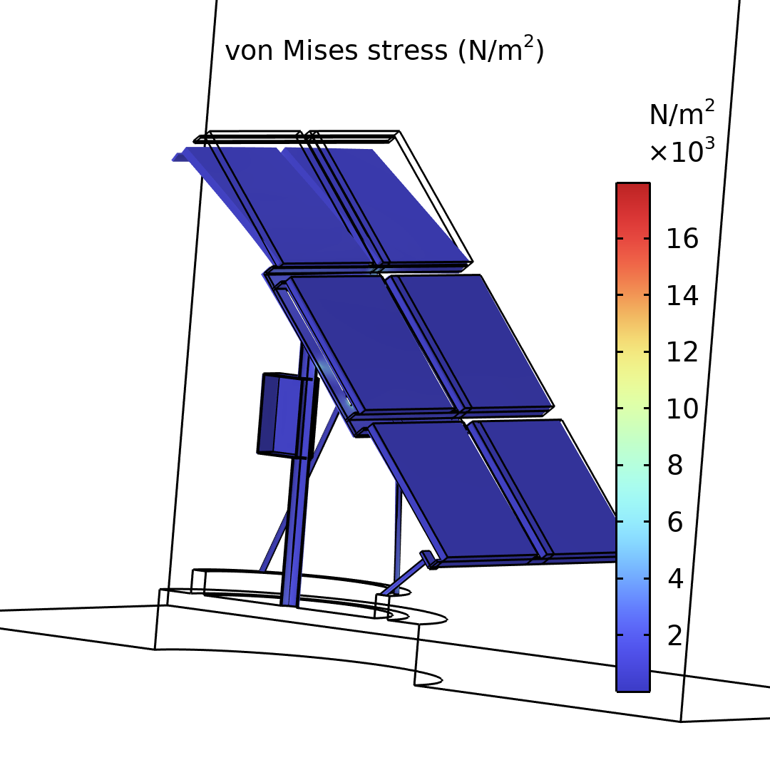
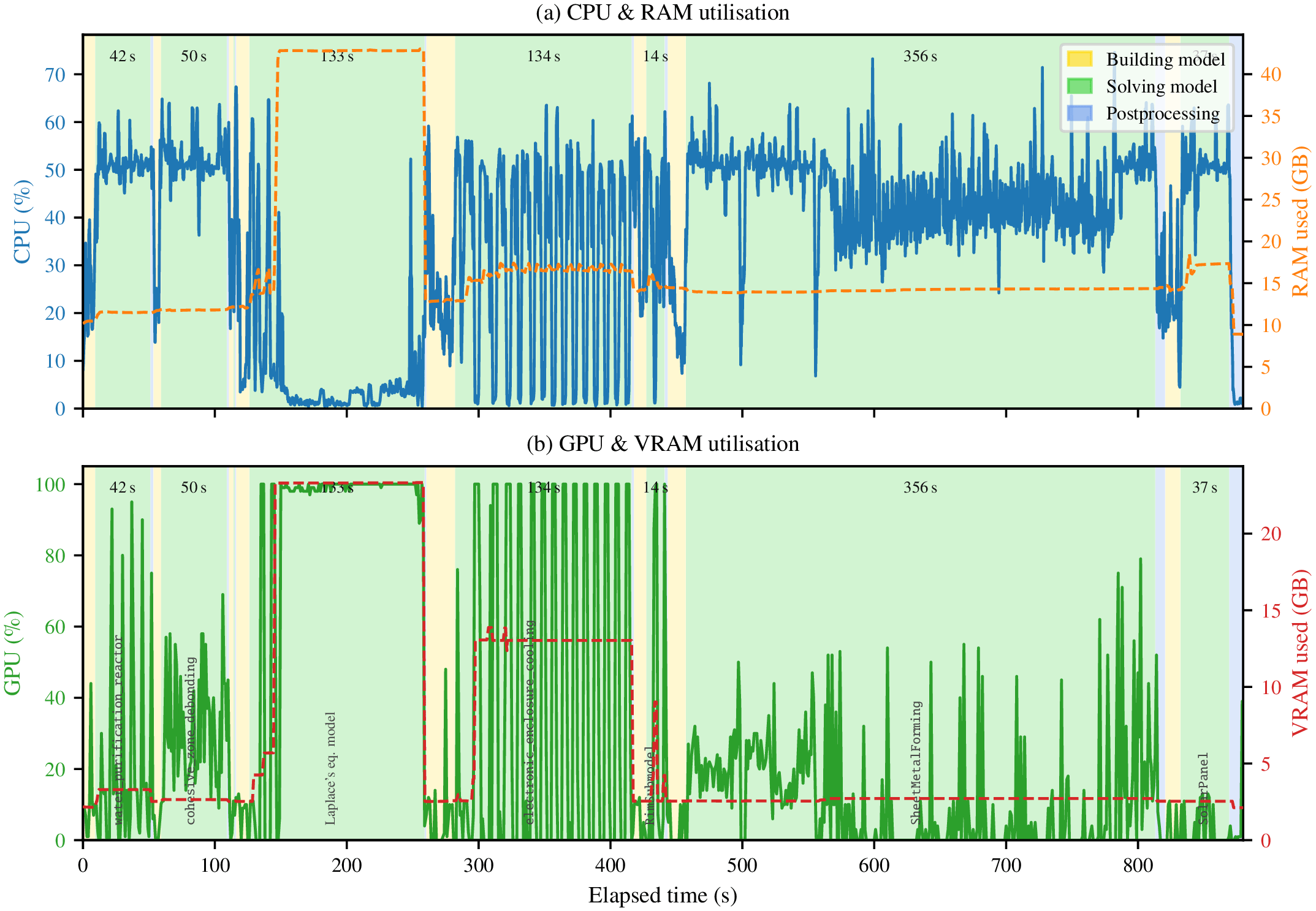
Fig 1. GPU utilization observed across benchmark models when using the CUDA Direct Sparse
solver.
B. GPU utilization
One of the observations from the benchmark was that GPU utilization varied substantially from model to model when running cuDSS. For all models except Laplace’s equation model, utilization remained below 100%, while CPU utilization also stayed relatively high.
C. Meshing on different architectures
One issue with meshing is that the algorithm is not fully consistent across different operating systems or across different processor architectures such as AMD and Intel.
To obtain a fair comparison between systems, the mesh was stored in the COMSOL application and then loaded for each test so that there was no mesh variation across very different hardware and software environments. As a result, the solver comparisons were carried out on identical meshes rather than on meshes regenerated separately on each platform.
D. Systems tested
The COMSOL application was run on 12 different systems, with some systems tested under different operating systems (OSs), and with each system evaluated under at least a subset of the solver configurations.
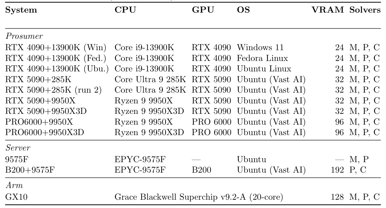
Table 1. Hardware and software configurations tested in the benchmark study. VRAM is reported in GB. Solvers: M=MUMPS, P=Paradiso, C=cuDSS.
Results
Three figures highlight the main aspects of the results: the overall performance comparison, the operating-system comparison, and the speedup obtained on each system when running on the GPU with cuDSS rather than on the CPU with Pardiso. The SolarPanel model is shown as a reference workload, but because it remains on an iterative multigrid solver, variation in that case reflects platform behavior rather than changes between the direct solvers.
To establish a baseline, we selected a capable but slightly older system as the reference configuration. Table 2 defines the standard baseline used for the comparisons in this section. The values shownin Figure 2 are normalized relative to the runtime of this reference system
A. CPU performance
1.x86 Prosumer vs. x86 Server vs. Arm
Here, x86 prosumer refers to desktop-class systems built around consumer CPUs and GPUs, x86 server refers to server-class systems with larger memory capacity and datacenter-oriented components, and Arm refers to the Arm-based Grace Blackwell platform tested in this study.
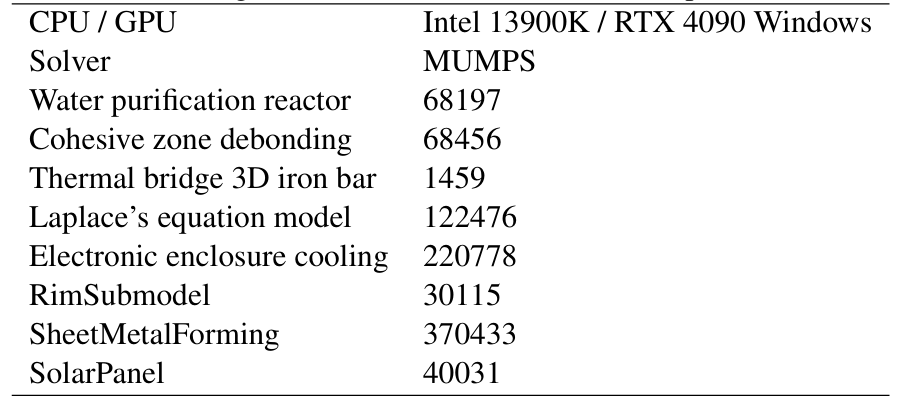
Table 2. Standard baseline timings used as the reference for the comparative results in milliseconds.
Figure 2, shows that the relative ordering is not identical across all models. The x86 prosumer platforms perform strongly, but they are ultimately limited in the model sizes they can run by the total amount of RAM that can be installed in those systems. One example is when Laplace’s equation model is run on GPUs with too little VRAM it forces the model into out-of-core memory, in this case regular RAM. While the x86 server platforms outperform most of the other systems, they do so at a price premium.
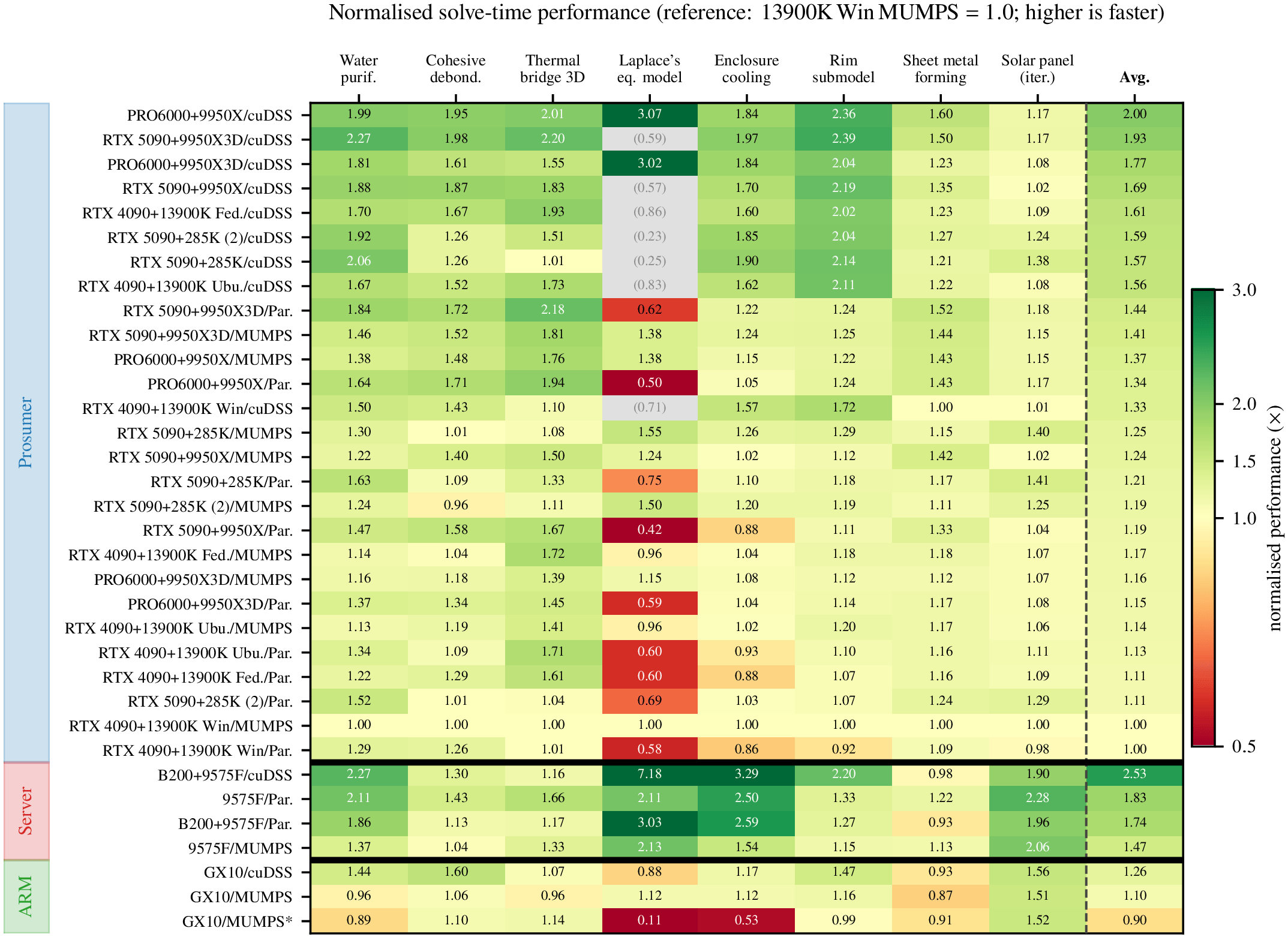
Fig 2. Normalized CPU performance for the x86 prosumer, x86 server, and Arm systems across the benchmark models. The Solar Panel model uses an iterative method that does not follow the solver changes between MUMPS, Paradiso, and cuDSS, so the variations in that column depend only on the CPU hardware on which it is run. Gray entries indicate out-of-core runs; these points are excluded from averages. GX10/MUMPS*was set to Paradiso, but COMSOL defaults to MUMPS with Pivoting perturbation when on ARM.
However, when absolute speed is the primary concern, they perform best. When the models become so large that they no longer fit in the RAM of regular prosumer systems, server systems become indispensable. Arm systems are somewhat of a dark horse. They have been gaining market share over the last decade, but they may still be uncommon enough that not all niches are fully developed. The Arm processor tested here is also unusual in that it operates with a GPU, shared memory, and a very fast interconnect between the CPU and GPU. All of these differences reinforce the need to evaluate solver performance on representative application models rather than relying on a single synthetic benchmark.
B. OS system effect
Operating system choice introduces measurable variation even when hardware, mesh, and solver settings are held fixed. Differences in driver behavior, math-library implementations, and memory-management overhead can shift total runtime enough to affect direct comparisons between platforms. For this reason, we treat operating system as an independent benchmark variable rather than as a purely incidental environment setting.
Figure 3 compares the same benchmark cases across the tested operating systems. The comparison helps distinguish genuine solver acceleration from platform-specific overhead and highlights where software-stack effects remain significant even before GPU acceleration is considered. For the operating-system comparison, the same hardware platform was used, so that the observed differences primarily reflect software-stack effects rather than hardware differences.
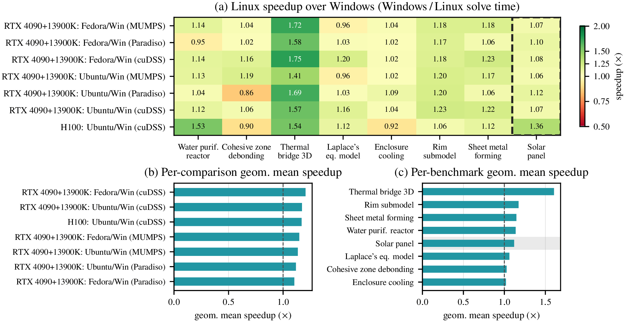
Fig 3. Runtime comparison across operating systems for matched benchmark models and solver settings
C. GPU Speedup
One of the main goals of this paper was to investigate the effect of adding GPUs to the system. As shown in Figure 4, there are large variations in the benefit of switching to the GPU solver, cuDSS, depending on the model and workflow. The speedup is greatest in the Laplace’s equation model case, where the GPU reaches full utilization, but substantial speedups can also occur in other models.
When running on a GPU, RAM is no longer the only parameter that determines the maximum model size. VRAM (video random-access memory) also plays a major role, because when a model does not fit in GPU memory it spills into system RAM, which greatly reduces calculation speed. In cases where Laplace’s equation model uses the cuDSS solver on an RTX 4090 or RTX 5090, performance becomes significantly worse because those graphics cards do not have enough VRAM. These data are therefore grayed out in the table, and the corresponding data points are excluded from the average. Prosumer GPUs typically do not provide large amounts of VRAM, and larger VRAM capacities are usually reserved for server-class GPUs, where they come at a premium price.
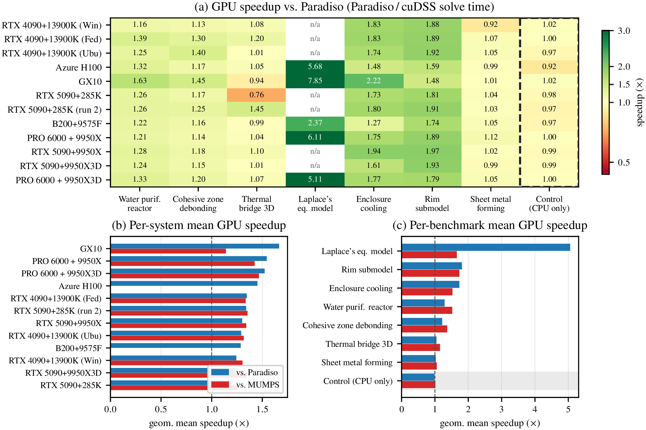
Fig 4. Solver speed up for GPU-enabled runs relative to matched CPU baselines
Discussion
The results indicate that GPU performance in COMSOL is not uniform; rather, it depends on numerical structure, memory-access patterns, and solver configuration. In general, meaningful speedups are possible when the model fits within the GPU’s available VRAM, but the performance gain may not always justify the added system cost. A powerful GPU alone does not guarantee strong results if it is not paired with a capable CPU. Therefore, rather than investing only in an expensive GPU, it may in many cases make more sense to invest in a better-balanced system with a stronger CPU. When absolute speed is the primary goal, however, the best results are achieved by pairing a high-end CPU with a high-end GPU.
If performance is critical and price is no issue then the best performance comes from pairing a high performance GPU (Nvidia B200 in our test) and a CPU that has both many cores and good single core performance (AMD 9575F in our test). Not all physics/models gain from many cores, but all gain from faster single core speed.
Choosing the right operating system can also provide substantial gains. Depending on the specific model, it is possible to achieve around a 20% increase in performance by choosing Linux rather than Windows on otherwise similar hardware. One limitation, however, is that COMSOL’s Application Builder is not available on Linux, so depending on the user’s workflow, that may be a tradeoff they are not willing to make.
Some sources suggest that VRAM memory bandwidth on the graphics card is a key parameter to optimize. However, our tests do not indicate that it is a major contributor to COMSOL performance. One possible reason for this perception is that memory bandwidth is very important in large language model (LLM) workloads, and people may have drawn a parallel to COMSOL performance that does not fully hold. This misconception may also be reinforced by language models themselves, which can repeat bandwidth-focused guidance when asked about the most important hardware characteristic.
Conclusion
This study shows that COMSOL performance depends on the full system configuration rather than on any single component. GPU acceleration can provide substantial speedup, but the benefit is strongly model dependent and the problem needs to fit within available VRAM. CPU capability, RAM capacity, and operating system choice remain important, and in many cases a balanced system provides better value than investing in a GPU alone. Overall, representative benchmark models are essential for making reliable hardware and solver decisions in practical COMSOL workflows.
Independent benchmark by resolvent — COMSOL Certified Consultant.
COMSOL, COMSOL Multiphysics, and COMSOL Application Gallery are registered trademarks of COMSOL AB. This benchmark study is independent work by resolvent, it is not affiliated with, endorsed by, or produced in partnership with COMSOL AB. The analysis and conclusions presented are resolvent’s own.