In Process engineering mixing or reduction of inhomogeneity can be applied to solid, liquid, or gaseous mixtures. The process of carbonation, in which carbon dioxide (CO2) is dissolved in water (H2O), and produces sparkling water, is an example that most people can relate to. Many households have a soda maker that just pumps CO2 at elevated pressure into a container of water to generate soda; there is no impeller or other complex structure to aid the mixing.
Another familiar type of mixing is how best to dilute concentrated juice in water for a tasty and refreshing drink. You would typically use a spoon or something similar, to mix it adequately, simply pouring the concentrated juice into a glass of water does not blend it very effectively.
In this article, we scale up the process and examine some of the benefits, prerequisites, and aspects of simulating the mixing of miscible liquids in stirring vessels, a practice frequently used in the chemical and pharmaceutical industry.
Prerequisites for simulating mixing of liquids in stirring vessels in the Pharmaceutical Industry
Ideally, simulations should be applied early in the design of any new process line. Initially, it might be space-independent reaction kinetics. However, ultimately the idealized perfect mixed system and plug-flow condition need to be challenged, and a better understanding of the process line equipment is crucial for high-quality and yield process lines. The Finite-Element Method (FEM), which is a well-known simulation method, can be used to perform a high-fidelity analysis of individual process line components including mixers, connectors, distributors, and more. This is because it considers temporal- and spatial-dependent factors.
To simulate mixing with stirred vessels, it is recommended, as with testing, to start with a pilot-size vessel. This helps to accelerate the process of verifying the simulation setup that has been chosen and provides answers to issues like: Is the setup’s physics accurate captured/described, or do we need to include more detailed descriptions of the process; Is a stationary analysis adequate, or do we need a transient study.
On the one hand, we would like to include all physics we can think of influencing the system. On the other side, including all physics can significantly extend simulation times and memory consumption without necessarily having a large impact on the results. Thus, the role of the simulation engineer is to apply knowledge and experience and choose an appropriate level to adequately describe the system. To achieve this, increasing the number of iterations that are feasible within the allotted time is facilitated by a pilot-sized component.
The Reynolds number of the impeller is a good place to start. This informs us of the expected flow regime and if the flow may be roughly classified as laminar, transitional, or turbulent.
Difference between stationary and transient simulations
Depending on the fluid parameters and the quantities the simulation is supposed to emphasize, it can either be assumed that the simulation is stationary or transient. If there are any dead- or recirculation zones inside the stirring vessel, a stationary investigation can identify them. It can also, among others, be used to assess the impeller’s torque and power consumption. A stationary study can be used to understand the temperature distribution inside the vessel if heating or cooling pipes are present.
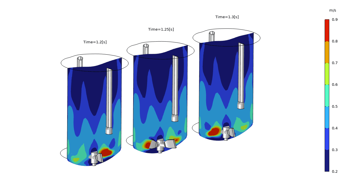
A transient simulation is required for transitory effects like mixing time, which is often of primary concern. It is beneficial to speed up the simulation while performing transient analysis with long simulation times by giving it a good initial value. An example is to begin a transient simulation with the solvent already in motion when adding a chemical species to it. Whenever one or more chemical species are added, and the mixing time is calculated, we may not be interested in the initial transient stirring of the solvent and instead use a frozen rotor approach to get an initial value for the transient study.
When reaction rate or fluid properties, such as viscosity change while mixing due to changing the chemical composition or temperature the system becomes coupled, and during a transient simulation, these quantities are updated based on the locale concentrations and temperatures while solving.
Process of testing the simulations
- Accessing the outcome: It is time to assess the outcomes after choosing the physical effects and governing equations and finishing the first simulation. It is time to scale up the mixer if test data is available and the simulation results demonstrate acceptable agreement. If the simulated findings do not match the test setup, a closer examination of the simulated and tested system is required. Any inconsistencies should be considered before continuing.
- Picking the right vessel: It’s not easy picking the right design for a stirred vessel. The size and shape of the stirring vessels, as well as whether and how many baffles should be used, are crucial factors. Some procedures may require heating or cooling, which is frequently achieved by adding piping inside the tank. The number of impellers, as well as their size and design, are important. Fluid in the stirring vessel can be distributed radially, up, or down depending on the impeller’s form. While some impellers produce significant shear stress, others do not.
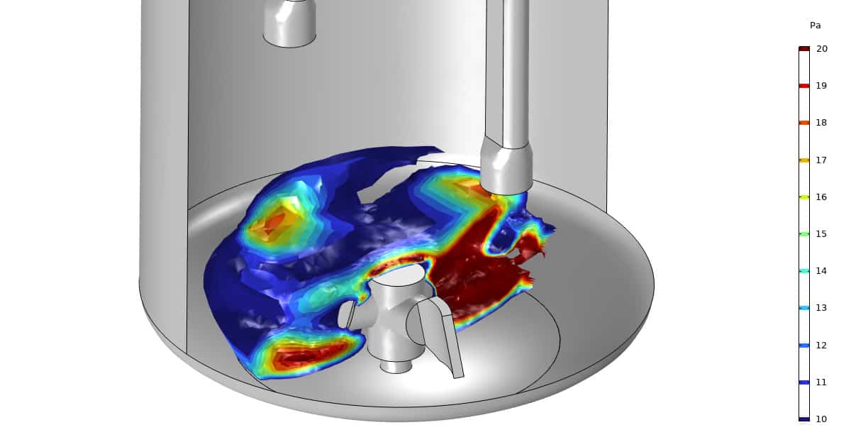
- Outcome: The desired outcomes can differ from project to project, but one that is frequently of importance is the shear stress the product experiences during mixing. It might be the amount of shear stress experienced over time or the maximum amount of stress experienced close to the impeller. Either the impeller speed or topology can be altered if the shear stress is too high.
Simulated torque and power consumption help in selecting the best machinery to drive the impeller.
The simulated flow field reveals dead- or recirculation zones that should be eliminated to maximize yield since they can prevent mixing.
Before constructing the mixer, hot or cold spots can be identified and fixed.
Summary
In conclusion, Multiphysics Simulations provide valuable insights into the complex mixing process. Visualizations of the simulation results make knowledge sharing between departments and colleagues much easier. For example, for identifying dead- or recirculation zones, too high or low shear stress regions, and other factors, resulting in higher quality products with less mixing time. All being candidates for saving electricity and increasing revenue in one go!